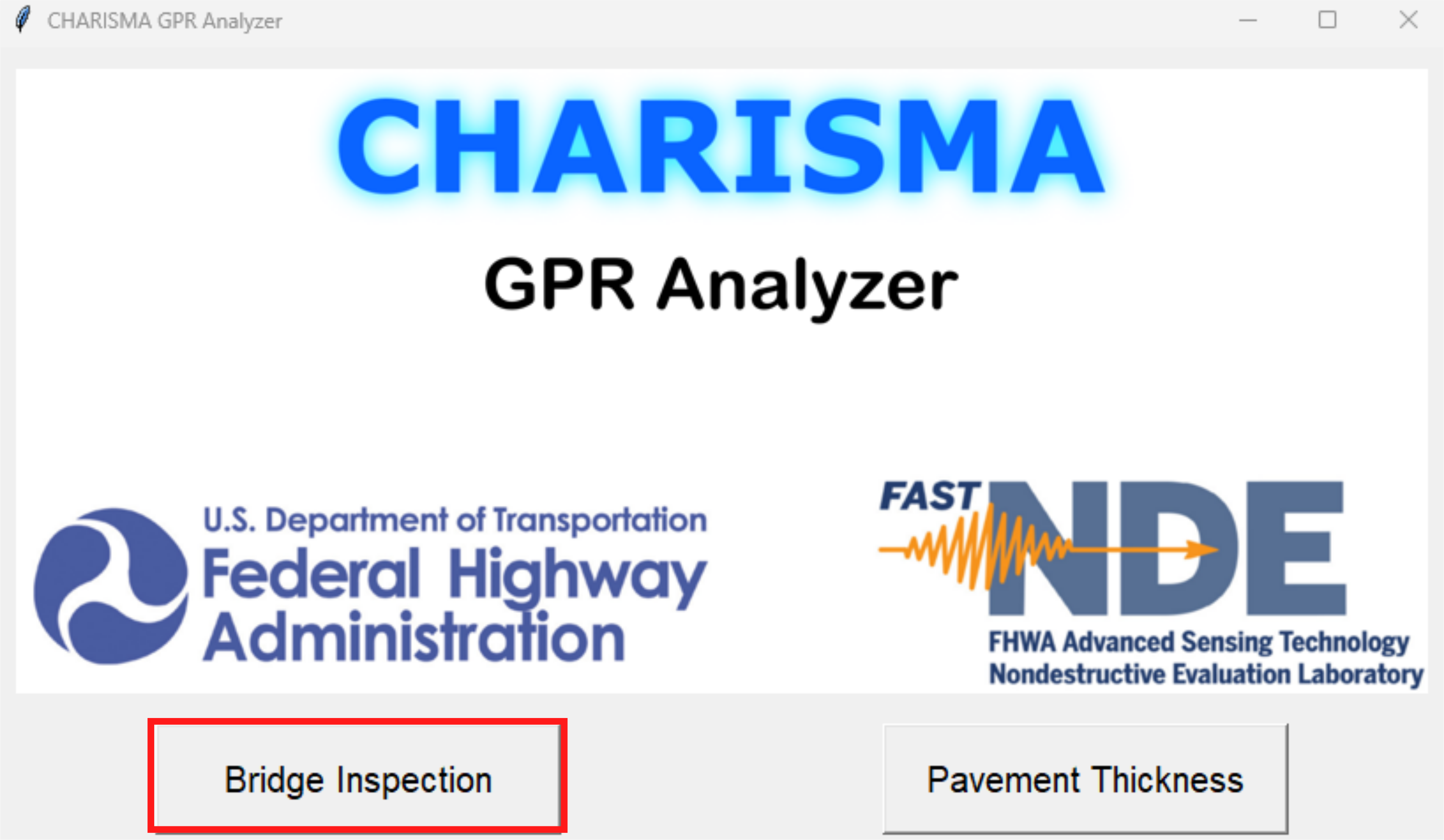
CHARISMA-GPR is a Python-based software designed to automatically process Ground Penetrating Radar (GPR) data for transportation asset management. It provides 2-dimensional contour maps required for the bridge inspection and pavement thickness measurement.
The software features a user-friendly Graphic User Interface (GUI) where users can easily input two key items: (i) the directory path of the GPR data and (ii) the GPR scanning configurations. Once the input is provided, CHARISMA-GPR outputs the contour maps, along with the raw data and the intermediate processing steps.
Users don’t need to understand the underlying code or have prior knowledge of GPR data processing—simply clicking a button gives asset owners the insights they need to make critical decisions about the maintenance and upkeep of infrastructure.
Each algorithm is validated through lab specimens and testing fields. The research team welcomes the community to use, test, and improve the software through the CHARISMA project. All data and code are available at the GitHub repository of CHARISMA. Future work will expand to other common NDE technologies for highway infrastructure inspection.
CHARISMA-GPR assumes a rectangular grid layout with linear GPR scans to generate a contour map. It accepts multiple GPR scan files in one directory, each representing a linear scan taken at regular intervals. These files will be processed to fill the grid space and create a contour map through interpolation.
We follow standard frameworks developed by ASTM and AASHTO. The data collection methods and device settings are well established in the documents. However, still, there are some unclear or vague statements in the data processing part, that lead to subjective interpretation. To address this, we conducted a comprehensive literature review on GPR data processing and selected only the most widely accepted and commonly used steps. Our software achieves full automation by following the necessary framework (time-zero, background removal, migration, dielectric constant characterization, and rebar mapping). Each step will use a fixed algorithm to output a consistent result.
CHARISMA-GPR creates a 2-dimensional grid space based on the user input and fills up this space with multiple GPR scans. In our software, you have the flexibility to define the x and y directions of the 2D contour map based on your perspective of the scan area. Since the orientation may vary depending on where you stand, you can choose which direction corresponds to the x and y axes. For example, if you are standing on the north side looking south, you might decide that the x-axis runs west to east, and the y-axis runs north to south. However, if you change your position—say, standing on the south side looking north—your definition of the x and y axes will flip. This shift in perspective can cause confusion if the directionalities aren’t clearly defined based on your view. To avoid this, we’ve made the configuration flexible, allowing you to set the axes according to your unique viewpoint, ensuring a user-friendly experience regardless of your orientation in the field.
After defining these axes, you’ll select the scan origin, which is the starting point for filling the grid. The origin can be any of the four corners of the rectangular area, depending on your setup. Once the axes and origin are set, you’ll choose the scan direction, which can either follow the x-axis or y-axis. Since there are four possible origins and two scan directions for each, there are eight potential configurations for how the grid is filled. Based on your selections, the software will process the GPR data and generate the 2D contour maps accordingly, ensuring that the output matches your perspective.
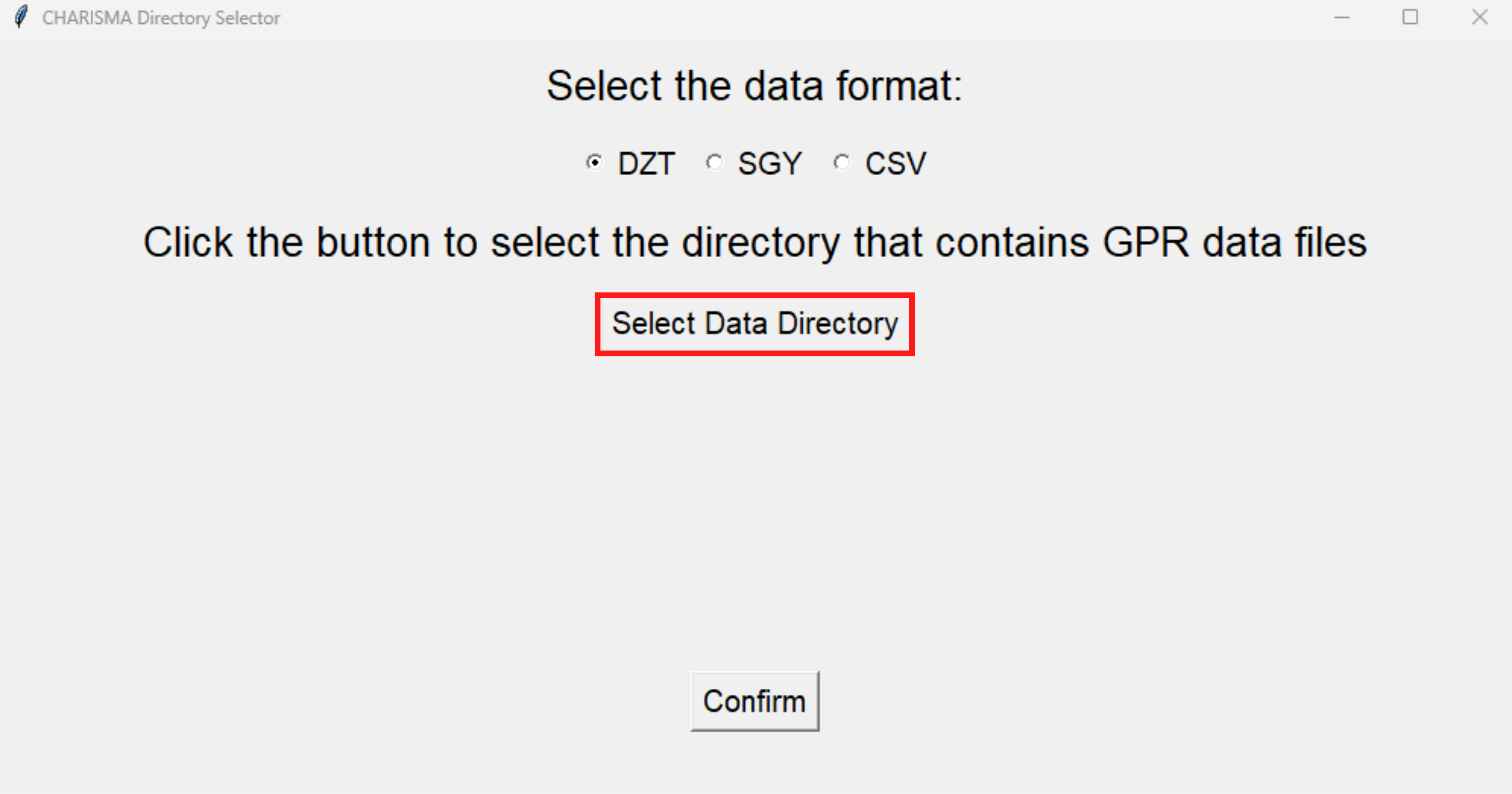
File Format Support: CHARISMA-GPR currently supports only the .DZT file format. Support for other formats, such as .SGY and .CSV, will be added soon.
Grid Space Assumptions: If the scanning area is not rectangular (e.g., trapezoidal or parallelogram), the contour map may show white spaces (no data to interpolate).
Single Channel Requirement: Currently, CHARISMA-GPR does not support multiple-channel DZT files. It only accepts a series of DZT files containing single linear scans.
Rebar Mapping Algorithm: The software employs the F-K migration algorithm for rebar mapping, which assumes that the dielectric constant of the subsurface materials remains constant throughout the entire area.
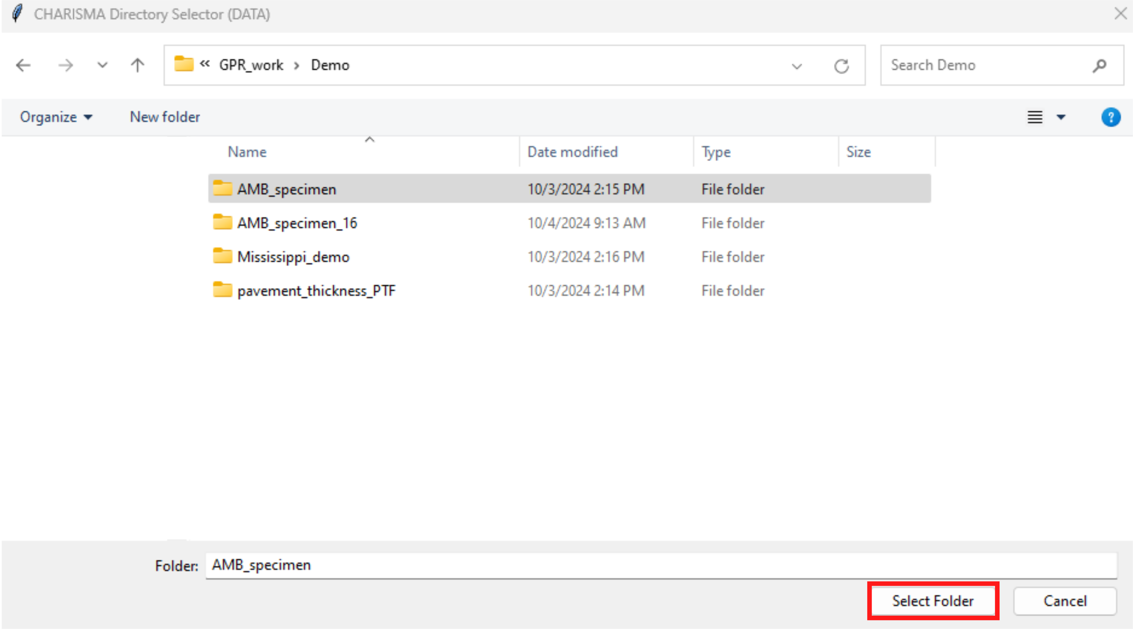
Directory Structure: Create a directory containing a series of single-channel .DZT files.
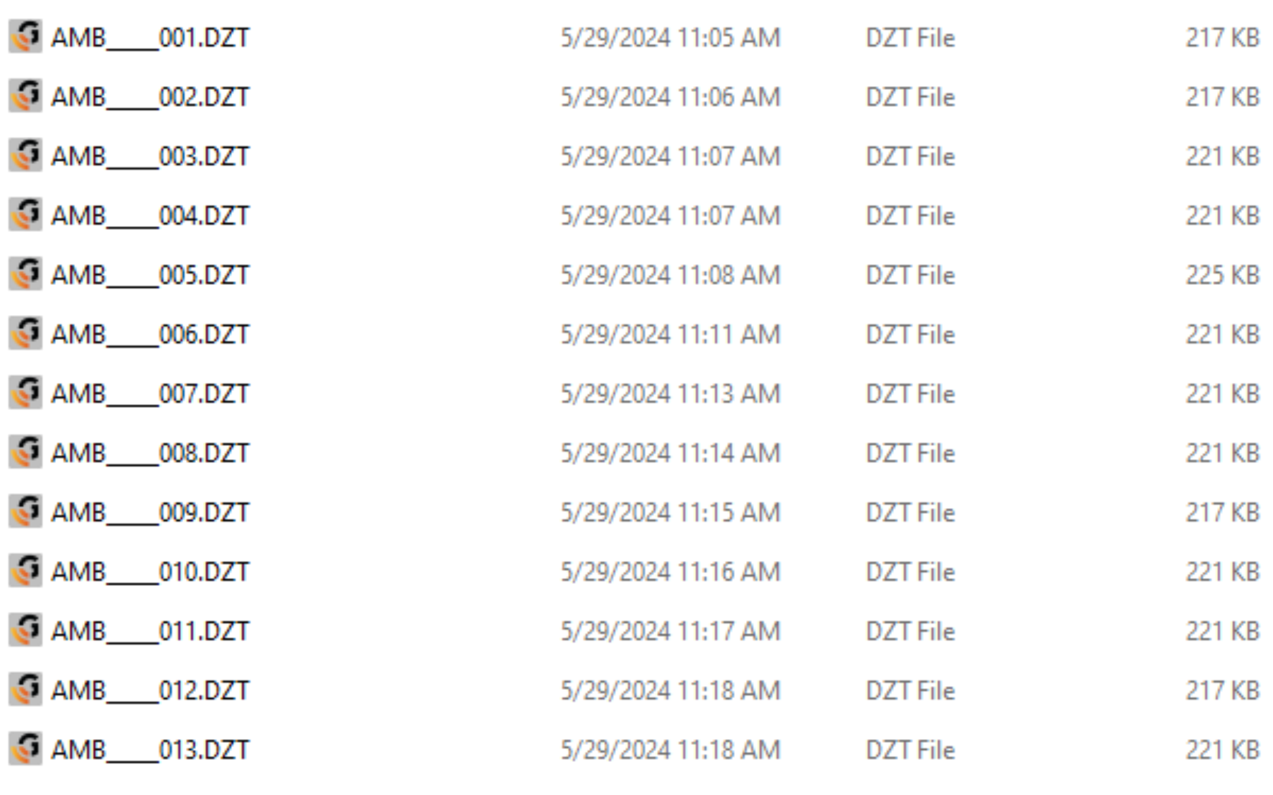
File Naming Convention: The file names should be ordered numerically using padded numbering (e.g., 001, 002, 003). Using a simple sequence like 1, 2, 3, … will change the order. Specifically, the order may appear as 1, 10, 2, 3, etc., because the number “1” is at the beginning.
Grid Space Information: You need to know the dimensions of the grid space, including the x and y distances in a specific unit, as well as the scan origin point.
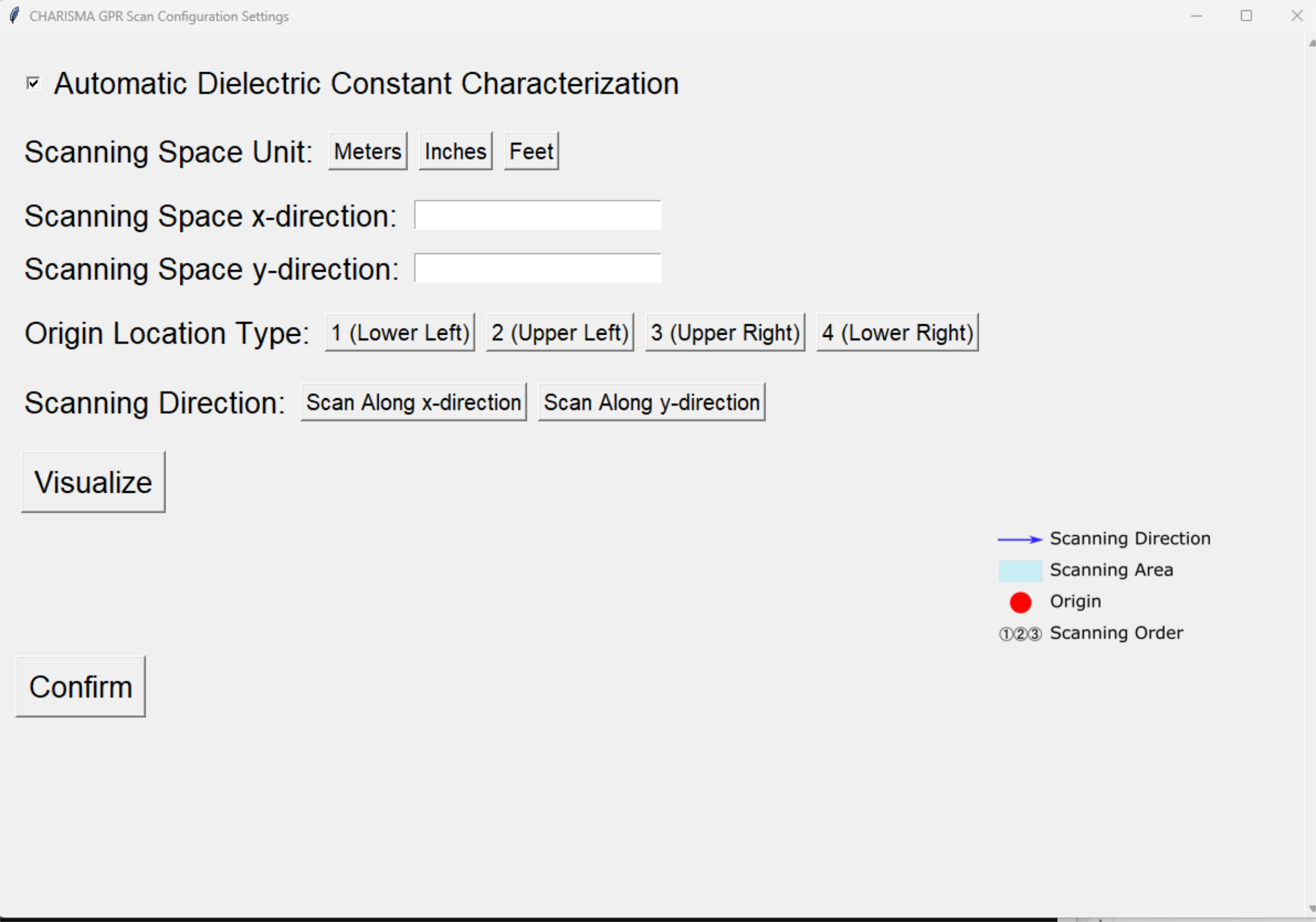
To manually set the dielectric constant, uncheck Automatic Dielectric Constant Characterization and enter your value. The automatic algorithm will still run for the reference, but your manual value will be used for data processing.
Choose the scanning space unit: Meters, Inches, or Feet.
Enter the x and y distance values for your scanning area. Imagine the scanned space as a rectangle, with x as the base and y as the height.
Select the origin based on the vertex from where you began scanning.
Choose the scanning direction: either along the x or y axis from your selected origin.
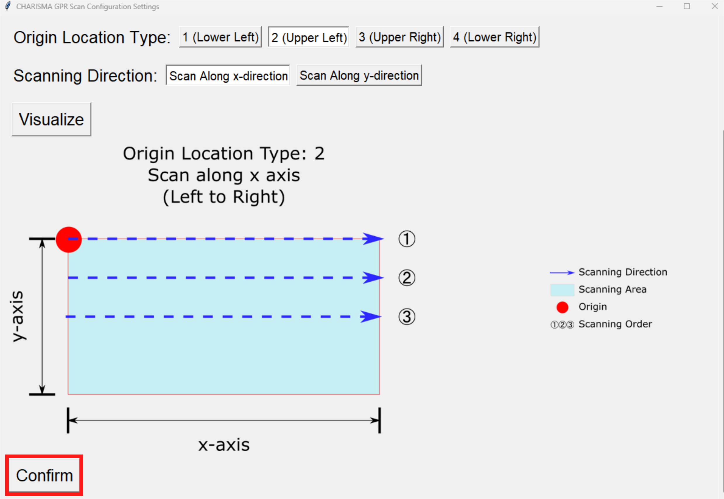
Click Visualize to verify your scanning configuration. If the schematic is not matching with what you expected, select other configurations and click Visualize again.
Figure 7: Clicking Visualization will show a schematic figure of your GPR scanning configuration.
Click Confirm to close the GPR Scan Configuration window.
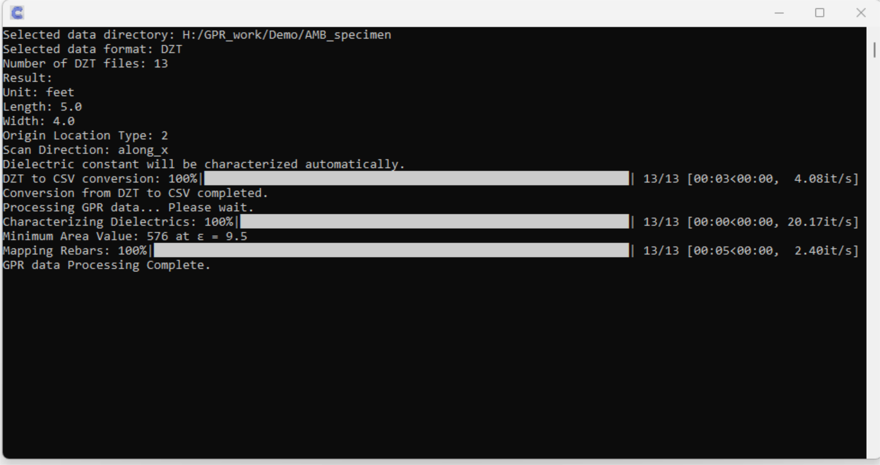
The Python logger will display the progress of data processing. Once complete, a new window will appear.
Figure 8: After confirmation, the software shows the progress through Python console.
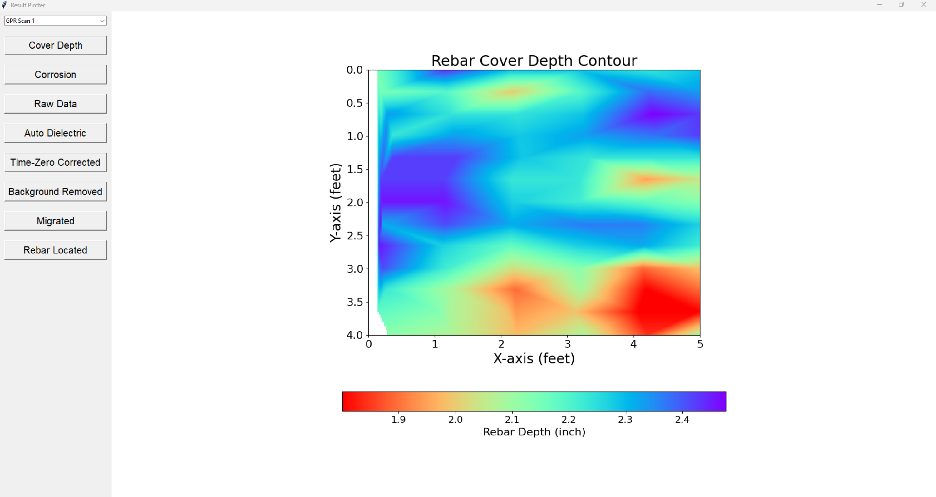
Use the left side buttons to view your results. Right clicking the image allows you to save it as a .PNG file.
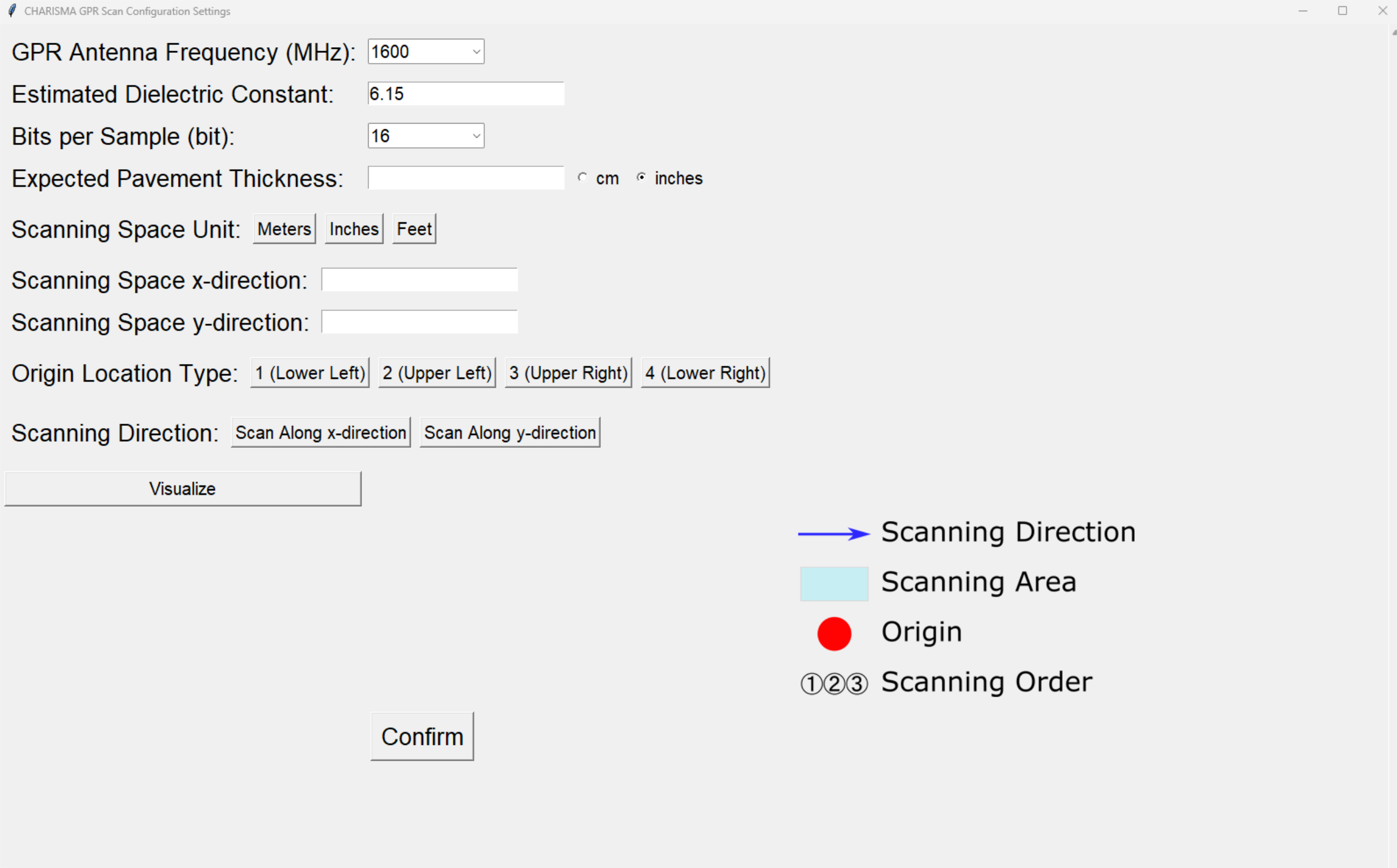
Enter the GPR antenna frequency, estimated dielectric constant, and bits per sample according to your GPR settings.
Enter the expected pavement thickness. This value sets the midpoint of the contour colorbar, indicating with some colors if the pavement thickness is above or below your expectations. Note that this value is used only for the colorbar reference, so it will not affect the data processing.
Choose the scanning space unit: Meters, Inches, or Feet.
Enter the x and y distance values for your scanning area. Imagine the scanned space as a rectangle, with x as the base and y as the height.
Select the origin based on the vertex where you began scanning.
Choose the scanning direction: either along the x or y axis from your selected origin.
Click Visualize to verify your scanning configuration. If the schematic is not matching with what you expected, select other configurations and click Visualize again.
Click Confirm to close the GPR scanning configuration window.
The Python logger will display the progress of data processing. Once complete, a new window will appear.
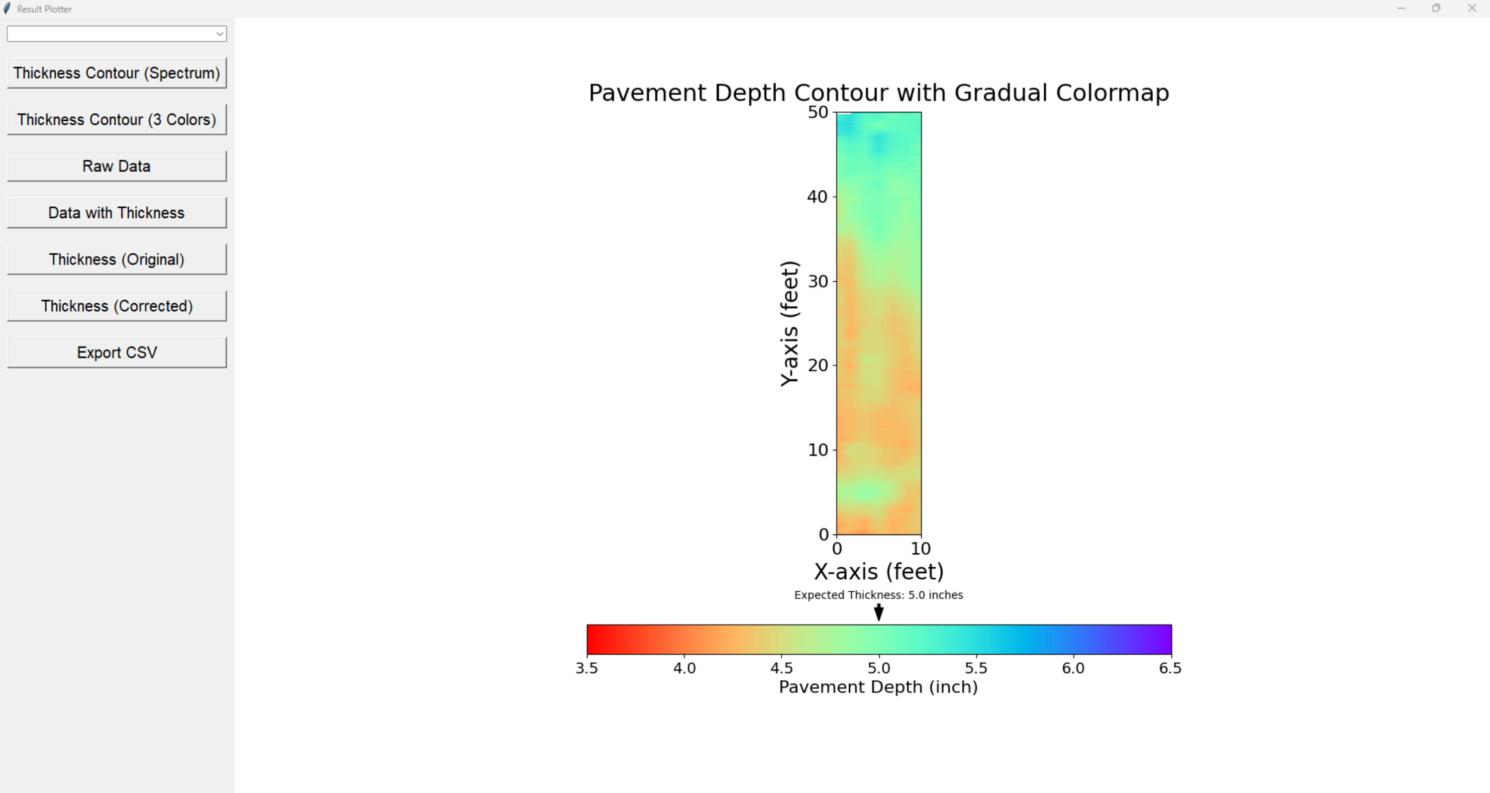
Use the left side buttons to view your results. Right-clicking the image allows you to save it as a .PNG file.
The upper-left dropdown menu lets you check the raw data and intermediate results, with the GPR scan files listed.
Click Export CSV to save the results as a .CSV file. A new window will open for you to enter the file name, and the file will be saved in the csv directory within the parent directory containing the GPR files.